This page was created to help observers and staff appreciate the design limitations of the current Q-band receiver. Hopefully, prospective observers can use this information to write proposals that are technically better. Observers with accepted proposals might be able to better plan their upcoming observations. Staff members should be better able to help our visitors. And, staff should be able to better plan any improvements to the receiver.
This page is divided into the following sections:
The essential sections for all Q-band observers are: "Current Receiver Design", "Dynamic Scheduling and Planning for Good and Bad Weather" and "Bottom Line: Current Receiver Performance Including the Atmosphere".
The Q-band (40-52 GHz) receiver does not have the performance that we have been advertising in our various documents, user guides, and e-mails. There are a few reasons for the restricted performance:
|
|
|
|
|
|
|
We're currently addressing the low frequency performance of the receiver and hope to have that repaired by the end of summer 2006. We are also contemplating whether redesigning the polarizer would be worth the effort -- the atmosphere is highly opaque above 48 GHz, making science very difficult; a new polarizer would need to be redesigned; a new polarizer would require building a new dewer, and a new dewer would require nearly a complete receiver redesign. We are not contemplating adding the two missing beams -- we're assuming the risk and the extra telescope time if observers were ever to want to use the receiver for mapping projects.
The rest of this documents describes what astronomers should expect out of the current receiver and the atmosphere over Green Bank. I'll be adding in the future a description of the expected future performance.
The weather affects observations at Q-band in three ways: winds affect the telescope pointing, differential heating/cooling affect the telescope pointing and efficiency, and atmospheric opacity affect the received signal and the system temperature.
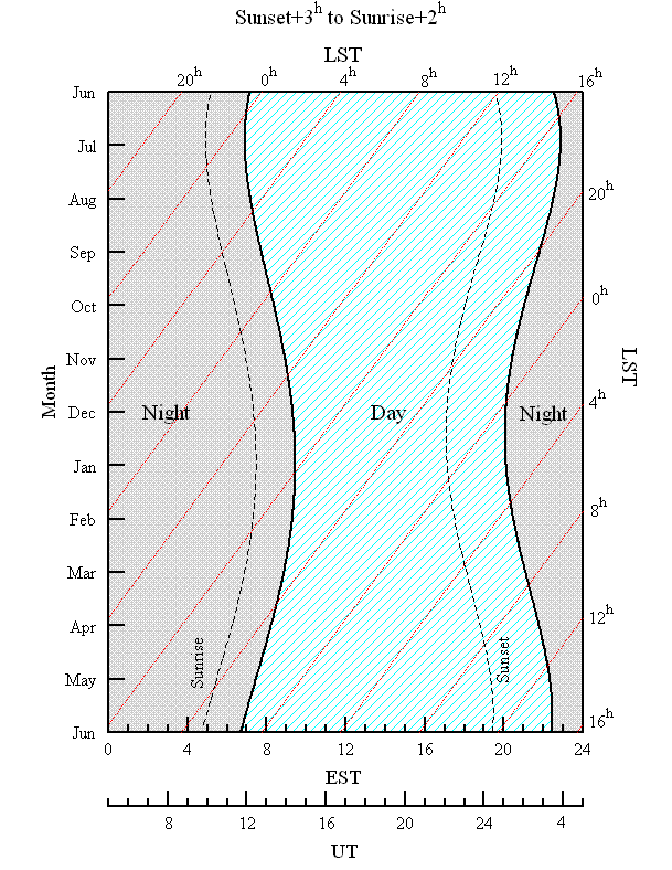
Differential heating and cooling of the telescope alters the surface of the telescope, resulting in poor telescope efficiencies, and 'bends' the telescope, resulting in rapidly-changing pointing. A goal of the Precision Telescope Control System (PTCS) is to measure and correct the telescope surface and pointing for these thermal affects. The PTCS has made a significant improvement with the introduction of "Dynamic Corrections". Even so, the current PTCS recommendations are that, for best work, Q-band observing should only be done at night, from 3 hours after sunset to 2 hours after sunrise. As the work of the PTCS continues, we can expect that the recommendations against daytime observing will be relaxed somewhat.
From October 1 to the end of April, a typical Q-band 'season', there's about 2750 'night-time' hours, about 54% of the total time. The following graph depicts the range of UT and LST for 'night-time' observing.
Winds tend to buffet the telescope and, to a lesser extent, set the feed arm into motion. Another goal of the PTCS is to increase the wind speed under which the telescope pointing is good at high frequencies. The current recommendations from the PTCS can be found at: https://safe.nrao.edu/wiki/bin/view/GB/PTCS/PointingFocusGeneralStrategy.
Currently we have determined that the conditions for "usable" performance at Q-band (<10% rms flux errors) result when the wind is less than approximately 5 mph. Although the pointing accuracy may be relaxed in some circumstances (e.g., when observing an extended source). Therefore, two characteristic wind speeds at 5 and 10 mph are used in the plots below.
The fraction of time when wind speeds are this low are illustrated in the above figure which shows the cumulative percentages when wind speeds are below a certain value. The data were for October 1, 2004 to April 30, 2005.

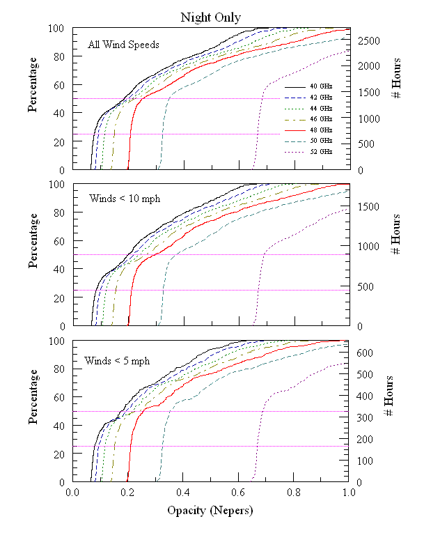
Since each year the weather trends can be different, these statistics, which are for just one season, shouldn't be too widely quoted. Note that there's very little difference between day and night time wind statistics.
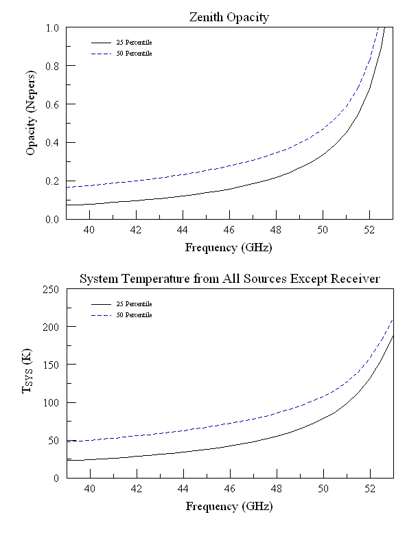
The 40-52 GHz band extends from frequencies where the opacity is relatively low to very high. The high frequencies are dominated by Oxygen absorption, the low by water vapor. Opacities from hydrosols (water droplets in fog, clouds, rain, ...) affect all frequencies but with 52 GHz affected about 70% more than 40 GHz. At 40 GHz, zenith opacities can be as low as 0.06 nepers on very cold, dry winter days while, at 52 GHz, the zenith opacity will never be lower than 0.65 nepers. The following two figure shows the cumulative statistics for opacity from the Oct 1, 2004 to April 30, 2005 season under various wind limits and for day plus night and just night observing. The opacities were calculated using the method described on my "High Frequency Weather Forecasts" web page.
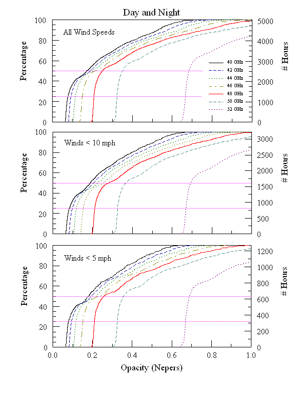
In all cases at all frequencies, the opacity curves have a significant change in slope at about 40-60%, with the curves having a very steep slope below the break point and a more gradual slope above. Note, in particular, that the curves are nearly vertical below about the 25% marker. Physically, the opacity from Oxygen dominates below the break point while water vapor and hydrosols dominate above. The steep-sloped curves below the break point show that Oxygen-dominated opacities do not change much with local weather conditions.
With our current implementation of "Dynamic Scheduling", one has double the chance of observing under 'good' weather. Thus, one can safely expect to be observing almost always with opacities that are at or below the 50% marker in the above figures. And, observers can anticipate that half of the time they will be observing with opacities below the 25% marker.
Since the curves are nearly vertical below the 25% marker, and since dynamic scheduling implies observations will seldom happen when the opacity is above the 50% marker, I'll use the opacities at the 25% and 50% to illustrate the range of weather conditions that observers should use for their planning and noise estimates.
Note that the opacity statistics don't change significantly from day to night or for various wind criteria. That is, since the statistics for wind speeds are mostly independent or uncorrelated with those for opacity, the simple product of the two statistics should describe the fraction of the time or number of hours that can be successfully used at Q-band. Since wind speed statistics are more restrictive than those set by atmospheric opacity, our current implementation of dynamic scheduling, and doubling an observer's chance of having good weather, is significantly insufficient.
Atmospheric opacity hits observing twice -- it attenuates the astronomical signal and it increases the system temperature due to atmospheric emission. The first of the following plots show the expected zenith opacity as a function of frequency for the 25 and 50% opacity percentiles from the previous opacity graphs, as calculated using the method described on my "High Frequency Weather Forecasts" web page. The second plot is the contribution to the system temperature from the atmosphere plus all other causes (Cosmic microwave background, spillover, ...) except the receiver. I will show system temperatures that include the receiver in the next section.
As mentioned above, the current receiver has poor performance for one of its feeds at low frequencies (due to hardware issues) and poor performance at high frequencies (due to the cutoff frequency of the polarizer). The following plots show the engineer's measurements of receiver temperatures for the receiver's four channels (R1, L1 are the right and left channels for beam one, R2 and L2 the same but for beam two) as a function of frequency. Adding these receiver temperatures to the above plot produces the expected zenith system temperatures for the 25% and 50% percentile opacity conditions.
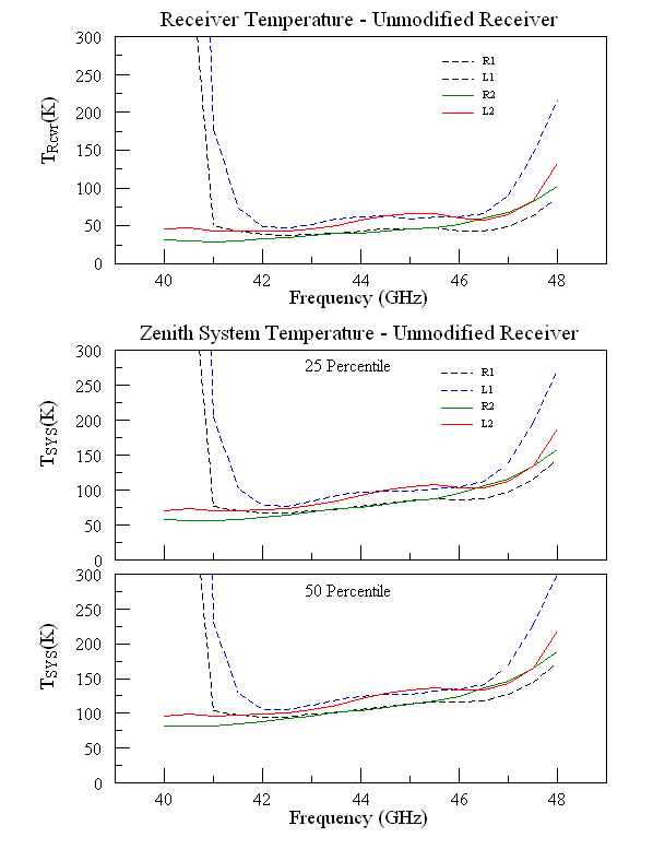
Essentially, the receiver can be used as single beam receiver below 41.5 GHz and, therefore, NOD'ing (dual-beam) experiments can not be done below this frequency. Above 46.5 GHz, one can still NOD but should expect only 3/4 of the data having useful system temperatures due to the poor performance of the L1 channel. Between about 41.5 and 46.5 GHz, one can successfully NOD.
To further help observers plan their observations, the following graphs show the total system temperatures for the current receiver as a function of elevation and frequency for the 25% and 50% percentile opacity conditions.
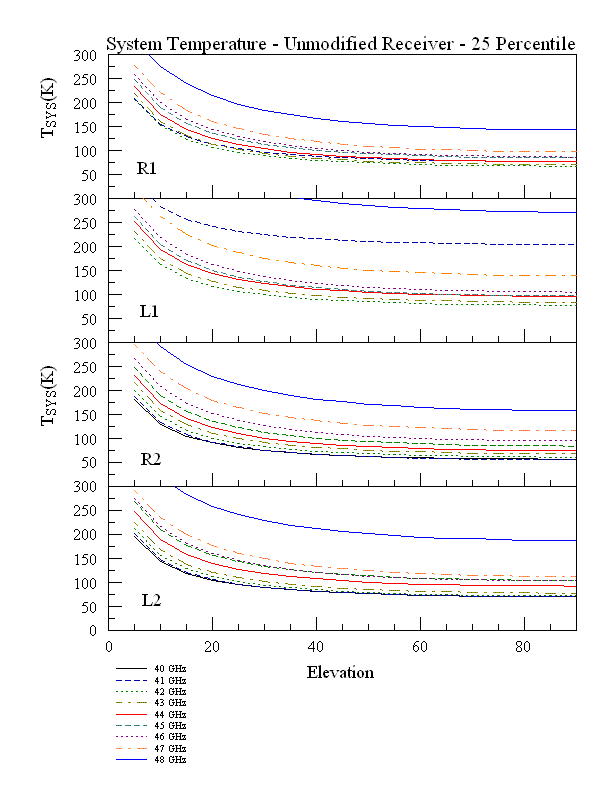
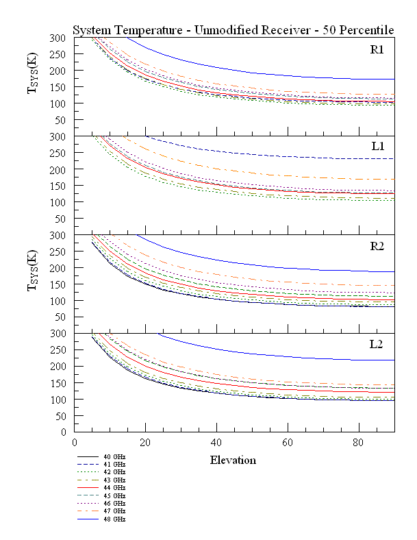
Observers proposing to use the GBT should use a Tsys that is close to that described by the 50% graphs for a conservative estimate of the time needed to achieve a certain noise level. Using the 25% graphs will produce an overly optimistic estimate of the necessary observing time but a fair fraction of our lucky observers will have such weather conditions.