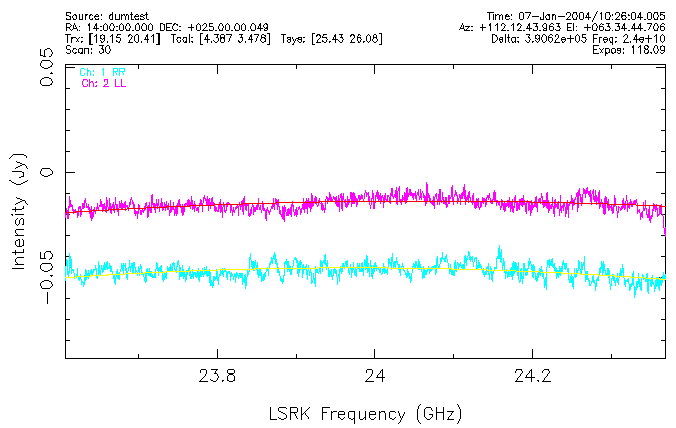
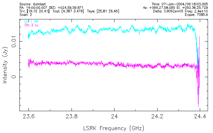
In this plot the smooth lines are the 2nd-order polynomial baselines that were fit, omitting channels near the edges of the spectrum. After subtracting the baseline, the rms flux density was calculated.
We used the GBT spectrometer in 800 MHz mode with 2048 channels per spectrum (channel spacing 391 kHz). Two spectral windows were used, centered at 24.0 and 24.8 GHz. Both beams were used and "nodding" observations were done, alternately putting the source in beam 1 and beam 2. We did not do beam switching. Temperature calibration was done by injection of a noise cal signal at 1 Hz.
A "dummy" celestial position was tracked: RA=14:00 hours, DEC=25 degrees. The telescope elevation was about 50 degrees. Each nodding pair consisted of two minutes integration, i.e., a total of 4 minutes on-source integration time for each pair. Thirty nodding pairs were done, for a total of two hours integration time.
The nodding scans were reduced using Jim Braatz's "reduce.g" program. The "reduce" program converted temperature to flux density assuming an aperture efficiency of 0.55 and an atmospheric tau = 0.05.
The configuration file used to set up the observation may be seen here.
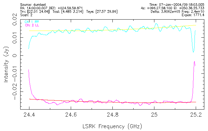
A typical reduced spectrum from one nodding pair is shown in
the following plot.
In this plot the smooth lines are the 2nd-order polynomial
baselines that were fit, omitting channels near the edges of
the spectrum. After subtracting the baseline, the rms flux
density was calculated.
In this way the rms was calculated for a single nodding pair, for the average of two pairs, 4 pairs, and so forth. As a final step, the data from all scans were averaged together and the spectra at the two frequencies were averaged to give 4 hours of effective integration time.
This final averaged spectrum (equivalent to 4 hours
effective integration time) is shown in the next plot.
| Integration Time | rms in 24.0 GHz band | rms in 24.8 GHz band | Calculated rms | ||
|---|---|---|---|---|---|
| (minutes) | RCP (mJy) | LCP (mJy) | RCP (mJy) | LCP (mJy) | (mJy) |
| 4 | 4.63 | 2.82 | 3.89 | 3.00 | 1.73 |
| 8 | 2.01 | 2.00 | 2.94 | 2.73 | 1.22 |
| 16 | 1.34 | 1.92 | 2.18 | 1.79 | 0.86 |
| 32 | 0.95 | 0.97 | 1.40 | 1.15 | 0.61 |
| 60 | 0.76 | 0.72 | 1.07 | 0.99 | 0.45 |
| 120 | 0.59 | 0.47 | 0.81 | 0.61 | 0.32 |
| 240 | 0.50 | 0.34 | 0.22 | ||
These data are plotted in the following graph.
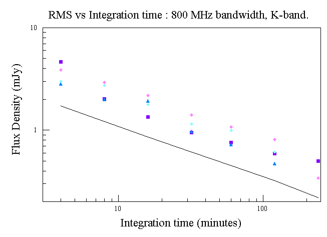
One may note that the measured RMS is decreasing with total integration
time as expected, but that the values are about two times what is
predicted by the radiometer equation.
The plots show small ripples of with width of about 50 MHz. The
size of these ripples seems to be decreasing with integration time.
The rms values after subtracting a 2nd order polynomial and avoiding the end regions of the spectra are tabulated in the following table:
| #channels Smoothing | RCP (mJy) | LCP (mJy) |
|---|---|---|
| 1 | 1.04 | 0.87 |
| 4 | 0.95 | 0.71 |
| 16 | 0.84 | 0.58 |