Dynamic Range Tests on Cass A
October 25, 2003
F. Ghigo, NRAO-Green Bank
The feasibility of mapping Cass A and its surroundings was
tested by doing scans across Cass A and across
weaker sources to see how linear the response
of the system is to a wide range of power levels.
System Components
- Front end low-noise amplifiers (LNAs)
- IF power range in Prime Focus receivers: 0.1 - 9 v ?
- Input to optical drivers: IF power range in IF Rack: 0.1 - 9 v ?
- Input to total power detectors in IF rack: 0.1-9v ?
- Input to SpectralProcessor: -4 to -34 db ??
Table 1. Journal of Observations: 410 MHz, October 19, 2003
| Scan# |
Source |
type of scan |
levels |
| 4-7 |
3C286 |
peak/point |
normal on background |
| 9 |
Cass A |
Scan 5 deg in RA |
set for peak of Cass A |
| 10 |
Cass A |
scan 5 deg in RA |
set for peak of Cass A |
| 11 |
3C286 |
scan 5 deg in RA |
set for peak of Cass A |
| 12 |
3C286 |
scan 5 deg in RA |
set for peak of Cass A |
Levels: "normal" levels means power in Prime focus receiver and
IF Rack is set to nominal 1v
and Spectral Processor to nominal -11db inputs when off source.
"set for peak of Cass A" means power meters in Prime focus
receiver and IF rack set at about 8v (near high end of allowable range)
and Spectral Processor inputs set to about -5 db.
Setup: Scans 9-12 used 20 MHz bandwidth centered on 410 MHz
for both the continuum(DCR) and Spectral Processor backends.
Used 0.1 second noise cal switching; Spectral Processor integration time
1 sec; scanning at 200'/min.
Results and discussion summarized
at the bottom of this page.
Peak Scans on 3C286
Peak Scans on 3C286 were done with normal level settings on off-source
background. Used normal Tcals (2.73 and 2.80 K).
These were done with the continuum backend for a 20 MHz band
centered at 410 MHz.
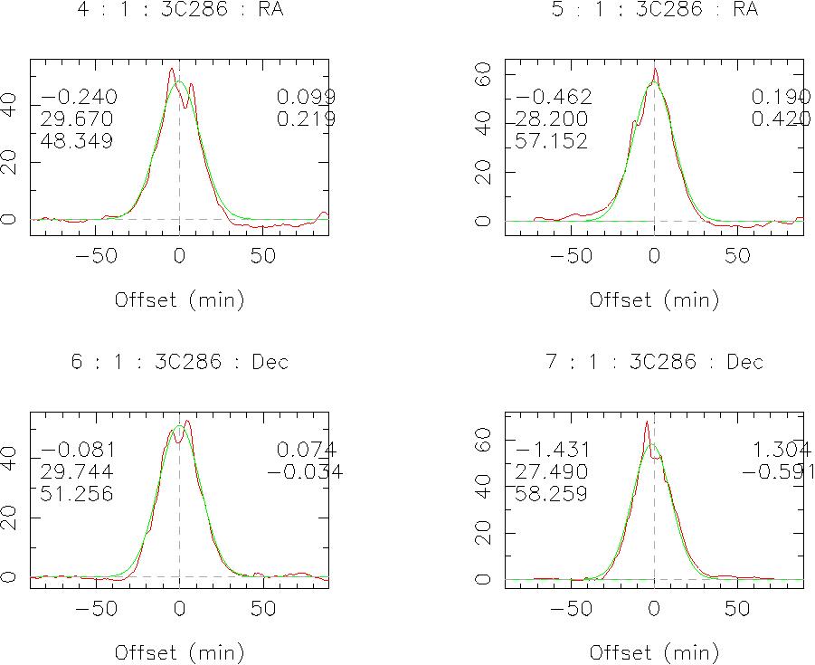
Scan 4 scans across the source in the +RA direction; scan 5 in -RA;
scan 6 in +DEC; scan 7 in -DEC.
The data were calibrated using the Tcals and are presented
in units of Kelvins.
In the plots, the observed data are shown in red and
the fitted gaussians in green.
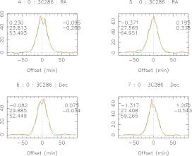 Plot 4A shows peaks on Xpol data.
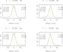 Plot 4B shows peaks on Ypol data.
Table 2. Summary of peak data.
| |
Xpol |
Ypol |
| Scan# |
Tsys(K) |
Peak(K) |
Tsys(K) |
Peak(K) |
| 4 |
62.1 |
53.5 |
60.3 |
48.3 |
| 5 |
62.4 |
65.0 |
59.6 |
57.2 |
| 6 |
63.6 |
52.4 |
58.2 |
51.3 |
| 7 |
63.8 |
59.3 |
58.3 |
58.2 |
Discussion
The flux density of 3C286, extrapolated to 410 MHz using the
data from Ott et al (1994), is 22.89 Jy.
The mean of the peaks is 55.7 K, which means the gain
is 2.4 K/Jy. This is too high -- the aperture efficiency
by design is 70%, which works out to a gain of about 2.0 K/Jy,
So the higher value of 2.4 is probably wrong.
The Tcals may be error, and should be closer to 2.3K rather
than the values we are using.
The variation of the peak values from one scan to the
next is large, but this may be explained by the fact that
variable RFI is in the 20 MHz band. One can see that the
peak are ragged -- rfi spikes are occurring in every peak.
This may be increasing the peaks and may explain the high
gains.
Spectral Processor Scans
The GBT scanned across Cass A for a 5 degree track centered on the
source at a rate of 200'/minute. The spectrum was dumped once per
second. Thus there were 90 spectra in each scan, and a 3.3'
spacing between spectra. Since the HPBW is about 30', there are
9 spectra per beam.
All spectra have 1024 channels.
The high Tcal was used (30.99, 32.98 K) and was switched
at a 10 Hz rate.
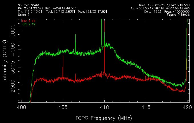
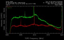 Plot 9A shows the first integration of Scan 9 across Cass A.
This is uncalibrated, in arbitrary units.
Plot 9A shows the first integration of Scan 9 across Cass A.
This is uncalibrated, in arbitrary units.
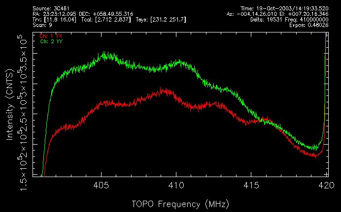
 Plot 9B shows integration number 45, on Cass A.
Also uncalibrated. Any RFI is overwhelmed by Cass A.
Plot 9B shows integration number 45, on Cass A.
Also uncalibrated. Any RFI is overwhelmed by Cass A.
Processing the Spectral Processor Data:
After looking at many of the individual integrations,
we determined the rfi-free channels to be the following:
channel numbers 40-230, 280-470, 600-660, and 780-920.
For each of the 90 integrations, we averaged the
rfi-free channels, separately for the cal-on and cal-off phases.
We used the difference between the cal-on and cal-off
phases averaged over integrations number 5-30 and 60-88
(the integrations without the source) and divided by the Tcal
to get a scaling factor to convert to units of temperature.
The result, for scan # 9 is shown in the next plot.
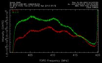
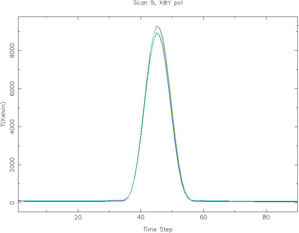
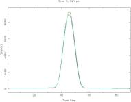 Plot 9C
shows the calibrated continuum data on Cass A.
The higher peak (red/green) is X polarization, and the
lower (blue) is the Y polarization..
Plot 9C
shows the calibrated continuum data on Cass A.
The higher peak (red/green) is X polarization, and the
lower (blue) is the Y polarization..
Similar processing for the remaining scans yields the
following plots:
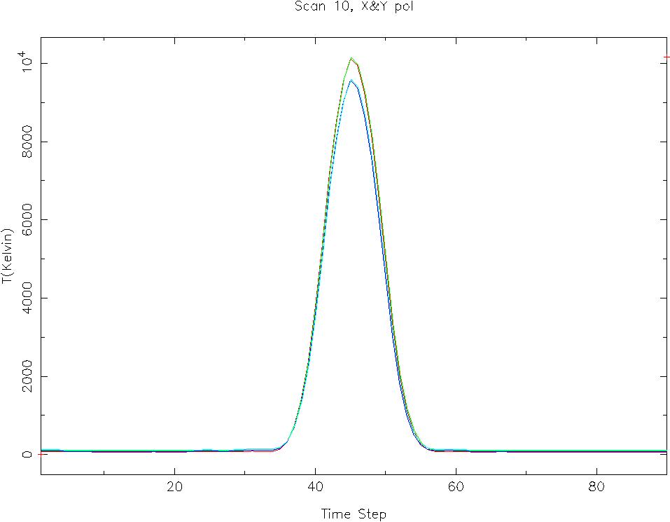
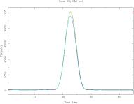 Plot 10A
A second calibrated scan across Cass A, done just the same
way as for scan 9.
Plot 10A
A second calibrated scan across Cass A, done just the same
way as for scan 9.
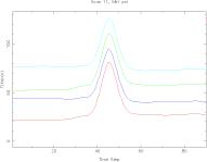 Plot 11A
Shows the scan across 3C286, processed the same way.
The red and green lines are the Cal-off and Cal-on phases,
respectively, for X polarization, and dark and light blue
are the same for Y-pol.
Plot 11A
Shows the scan across 3C286, processed the same way.
The red and green lines are the Cal-off and Cal-on phases,
respectively, for X polarization, and dark and light blue
are the same for Y-pol.
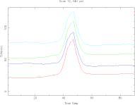 Plot 12A
Shows the second scan across 3C286.
Plot 12A
Shows the second scan across 3C286.
Summary of results
A summary of results from scans 9-12 is shown in the next table.
Tsys means the average baseline level for the cal-off phase.
Peak is the difference between the peak of the plot and Tsys.
Gain is Peak divided by the source flux density.
For the flux density of Cass A at 408 MHz in the year 2003,
we use 4223 Jy, based on Baars et al (1977).
For 3C286, we use 22.89 Jy, as described above.
Table 3
| |
Scan 9: Cass A |
Scan 10: Cass A |
Scan 11: 3C286 |
Scan 12: 3C286 |
| |
Xpol | Ypol |
Xpol | Ypol |
Xpol | Ypol |
Xpol | Ypol |
| Tsys (K) |
62 | 73 |
62 | 77 |
23 | 41 |
23 | 40 |
| Peak (K) |
9340 | 8840 |
10046 | 9480 |
58 | 53 |
55 | 50 |
| Gain (K/Jy) |
2.21 | 2.09 |
2.38 | 2.24 |
2.53 | 2.32 |
2.40 | 2.18 |
Discussion
- We don't worry about the gains being higher than the expected 2.0 :
this can be due to the assumed Tcal values being a little wrong.
We also don't worry about the difference between the X-pol and
Y-pol data since gains can be a little different for the
different polarizations.
- If everthing is nice and linear, we should expect the
gains derived from the two sources to be the same.
- If we take the average of scans 9 and 10 for Cass A, we
have the (X,Y) gains being (2.30 and 2.17 K/Jy).
- The average of scans 11 and 12 for 3C286 gives (2.47 and 2.25 K/Jy).
- Thus the gain scaling difference between Cass A and 3C286
is about 7% for X and about 4% for Y.
- But there may be systematic errors in our estimated fluxes.
Errors of the order 5% are probably to be expected.
- So as far as we can tell, the system is linear within about 5%
for objects ranging in flux density from 22 to 4000 Jy.
Let's also compare with the peak data (scans 4-7) done on
3C286. Here the gain is about 2.4 K/Jy, which agrees pretty well
with what we have in Table 3. So things are linear to 5% for
power levels ranging from normal to the low end of the range.
But some worries remain:
Why do we see variations of the order 10% from one scan to the next?
and why is the Tsys for the 3C286 scans much lower than for Cass A?
 Plot 4A shows peaks on Xpol data.
 Plot 4B shows peaks on Ypol data.
 Plot 9A shows the first integration of Scan 9 across Cass A.
This is uncalibrated, in arbitrary units.
Plot 9A shows the first integration of Scan 9 across Cass A.
This is uncalibrated, in arbitrary units.
 Plot 9B shows integration number 45, on Cass A.
Also uncalibrated. Any RFI is overwhelmed by Cass A.
Plot 9B shows integration number 45, on Cass A.
Also uncalibrated. Any RFI is overwhelmed by Cass A.
 Plot 9C
shows the calibrated continuum data on Cass A.
The higher peak (red/green) is X polarization, and the
lower (blue) is the Y polarization..
Plot 9C
shows the calibrated continuum data on Cass A.
The higher peak (red/green) is X polarization, and the
lower (blue) is the Y polarization..
 Plot 10A
  Plot 11A
 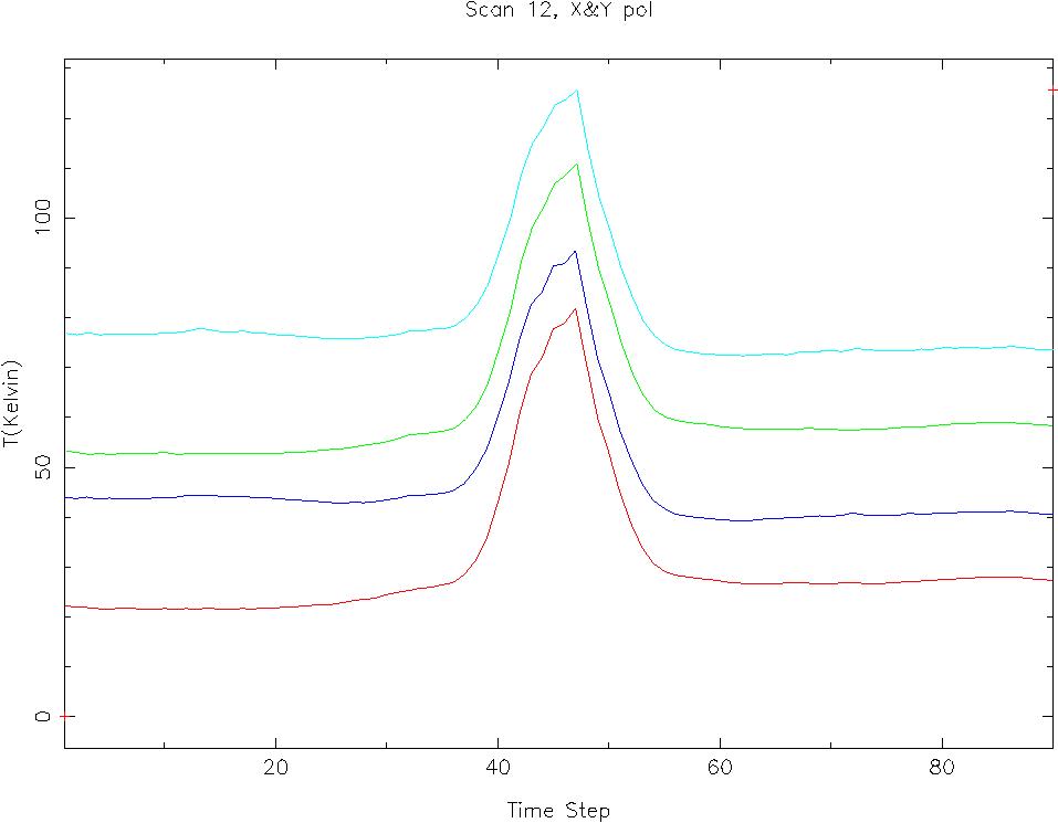 Plot 12A