GBT 450 MHz band RFI survey (Oct.03)
The 400-450 MHz band was observed while the GBT was doing
360-degree rotations in azimuth.
Summary of Data
| Date |
Band |
Project Code |
Backend(s) |
Types of Data |
| 2003 October 19 |
400-450 MHz |
TRFI450_OCT19 |
ACS(50MHz) |
Az rotation |
All ACS spectra done with 50 MHz bandwidth, 1-second noise switching,
2 second integrations, 1080 arcmin/min az rate (i.e, one 360 deg rotation
in 20 minutes).
Commentary on October 19 data.
The spectrometer was used in 50 MHz 9-level mode, with high
spectral resolution (32768 channels, i.e. 1.5 kHz channel spacing).
Scan numbers 15 and 16 were observed at night (2:45-3:30 AM local time),
and scan number 18 in the day (11:20 to 11:40 AM).
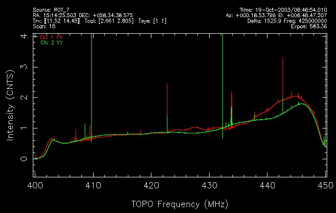
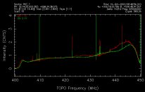 Plot 15A shows the uncalibrated data for scan
15 averaged over all directions. Major RFI spikes are seen at
409.8, 422.8, and 432-434 MHz.
Plot 15A shows the uncalibrated data for scan
15 averaged over all directions. Major RFI spikes are seen at
409.8, 422.8, and 432-434 MHz.
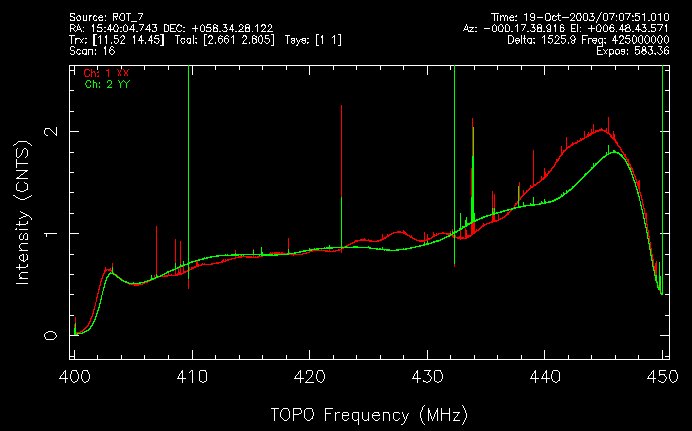
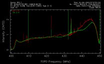 Plot 16A shows the uncalibrated data for scan
16 averaged over all directions.
Plot 16A shows the uncalibrated data for scan
16 averaged over all directions.
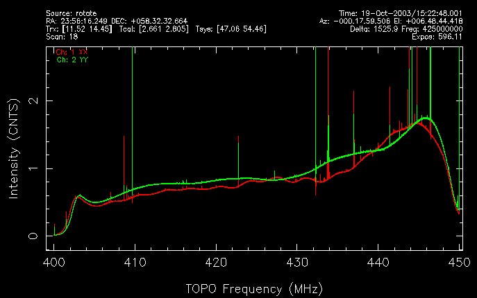
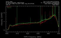 Plot 18A shows the uncalibrated data for scan
18 averaged over all directions. Major RFI spikes are seen at
443-446 MHz, 409 MHz, and 432 MHz.
Plot 18A shows the uncalibrated data for scan
18 averaged over all directions. Major RFI spikes are seen at
443-446 MHz, 409 MHz, and 432 MHz.
Doing median filter subtraction on all 599 integrations of 32786-channel
spectra proved to be too time-consuming. The spectra were averaged
to reduce the number of channels to 4096, increasing the channel
spacing to 12.2 kHz. The data were calibrated and converted to units
of Janskys (10**-26 Watts/sq.meter/Hz). A median-filtered baseline
was subtracted to flatten the bandpass. A 7-point median filter was
used on scans 15 and 16, 5-point on 18.
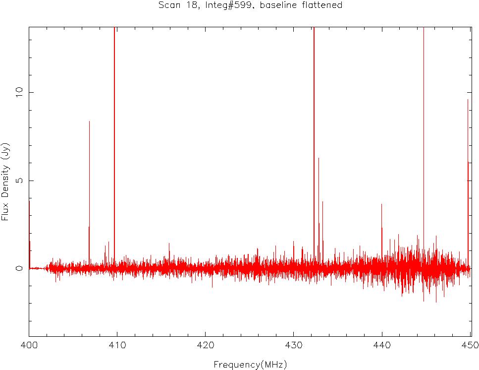
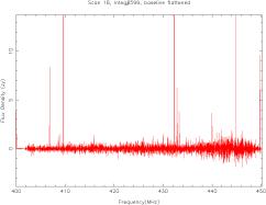 Plot 18B shows the calibrated data for scan
18 and integration number 599 after baseline flattening.
Plot 18B shows the calibrated data for scan
18 and integration number 599 after baseline flattening.
RFI spikes were identified as any data point exceeding 3.0 times the rms
in the baseline-flattened spectra.
 Plot 18C shows the same data as in plot 18B, with the
identified RFI spikes superimposed in green.
Plot 18C shows the same data as in plot 18B, with the
identified RFI spikes superimposed in green.
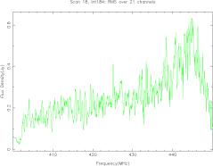 Plot 18D shows the typical run of rms with frequency,
for integration number 184. The rms was calculated over a
21-channel (256 kHz) window centered on each point in the spectrum.
Outliers above 2.6 times the rms were thrown out and the rms
re-calculated, so that the rms was not contaminated by RFI spikes.
This procedure was sometimes overwhelmed by very large and wide
RFI signals. In these cases, the rfi was so large that it was
identified anyway.
Plot 18D shows the typical run of rms with frequency,
for integration number 184. The rms was calculated over a
21-channel (256 kHz) window centered on each point in the spectrum.
Outliers above 2.6 times the rms were thrown out and the rms
re-calculated, so that the rms was not contaminated by RFI spikes.
This procedure was sometimes overwhelmed by very large and wide
RFI signals. In these cases, the rfi was so large that it was
identified anyway.
Note that the typical rms ranges from 0.2 to 0.6 Jy across the spectrum.
This may be a combination of the noise predicted by the radiometer equation
(0.12 Jy) and confusion (0.5 Jy).
The drop in rms at the band edges is probably bogus.
In fact, the change in rms across the band is probably bogus because
we used a single value for Tcal and deltacal for the whole band.
Download ascii files
Each of these files, when "gunzip"ed and un-tarred, becomes a directory
with 599(or 594) ascii files, each file contains 4 spectra taken at a particular
azimuth. The file has a header indicating the azimuth and time.
The data have been calibrated and are in units of Janskys, i.e.,
10**-26 watts per sq. meter per Hz.
The columns in the table are 1) frequency,
2) X polarization, 3) Y polarization,
and columns 4) and 5) is the same data with a median subtracted.
Scan 15, 594 2-second integrations.
Sweep from 0 up to 360 azimuth. Taken Oct 19, 02:46-03:06 AM (EDT) (34 MB)
Scan 16, 594 2-second integrations.
Sweep from 360 to 0 azimuth. Taken Oct 19, 03:07-03:27 AM (EDT) (34 MB)
Scan 18, 599 2-second integrations.
Sweep from 360 to 0 azimuth. Taken Oct 19, 11:20-11:40 AM (EDT) (34 MB)
 Plot 15A shows the uncalibrated data for scan
15 averaged over all directions. Major RFI spikes are seen at
409.8, 422.8, and 432-434 MHz.
Plot 15A shows the uncalibrated data for scan
15 averaged over all directions. Major RFI spikes are seen at
409.8, 422.8, and 432-434 MHz.
 Plot 16A shows the uncalibrated data for scan
16 averaged over all directions.
Plot 16A shows the uncalibrated data for scan
16 averaged over all directions.
 Plot 18A shows the uncalibrated data for scan
18 averaged over all directions. Major RFI spikes are seen at
443-446 MHz, 409 MHz, and 432 MHz.
Plot 18A shows the uncalibrated data for scan
18 averaged over all directions. Major RFI spikes are seen at
443-446 MHz, 409 MHz, and 432 MHz.
 Plot 18B
 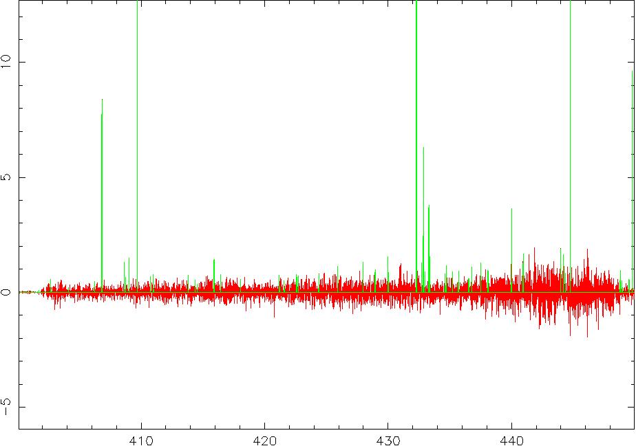 Plot 18C
 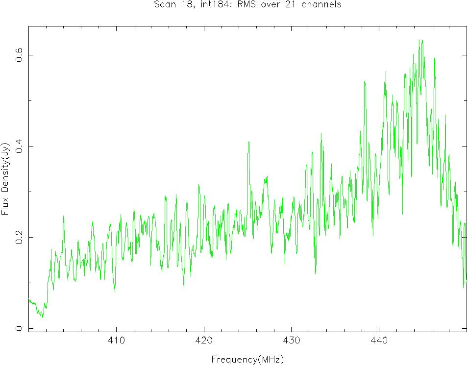 Plot 18D